Visual Quality Assessment of Composite Images: Compression-oriented Database and Measurement

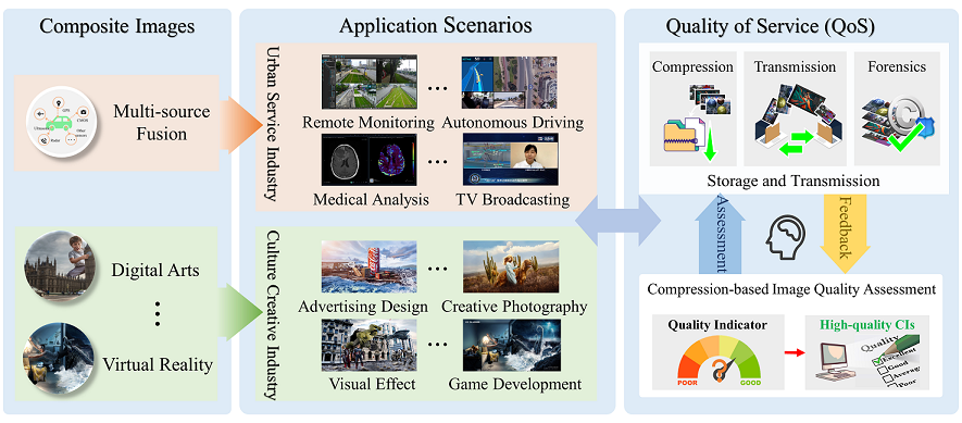
Fig.1: Typical applications of compression-oriented composite images.

We introduce how to build our ciCIQA database, which includes the following four steps: (1) data preparation and generation of compressed CI samples, (2) annotation of compressed CI samples, (3) processing of subjective results, and (4) statistical analysis of ciCIQA.

Table.1: Comparison of some mainstream IQA databases and the proposed ciCIQA.

(1) Data Preparation and Generation.

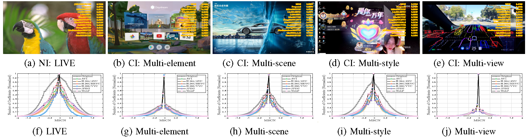
(1.1) Preparation of Raw CIs. We have collected and selected 100 representative CI source samples from different application scenarios, including generative AI, web design, video conference, poster design, medical image analysis, autonomous driving, security monitoring, e-sports, etc. Subsequently, we proportionally crop them into a resolution of 1920x1080 to ensure that they have the same size for the convenience of conducting subjective experiments. Based on their characteristics, we have summarized four main attributes such as multi-element, multi-scene, multi-style, and multiview, as shown in Fig.2.

a) Multi-element. Fusing various content styles (natural images, computer graphics, and cartoons) or content components (icons, text, lines, and charts) to create meaningful and engaging image content, which is commonly used in film posters, magazine covers, and web pages.

b) Multi-scene. Integrating various scenes or backgrounds (natural, urban, and cosmic), as well as different time and space dimensions (micro, macro, past, and present), to create diverse and rich image content, which is commonly seen in digital art, virtual reality, and TV broadcasting.

c) Multi-style. Combining different artistic styles (comics, abstract, and realism) or various artistic effects (filters, lighting, and shadow) to create unique and fantastical image content, which is commonly found in advertising, social media (i.e., UGC), and AIGC.

d) Multi-view. Integrating different perspectives or viewpoints (front, side, and top-down), and various modalities or dimensions (infrared images, depth maps, and point clouds) to provide a more comprehensive image representation of the target scenes or objects, which is commonly found in surveillance, e-sports, and autonomous driving.

These distinct attributes make the quality assessment of CIs more complex and challenging.

Fig.2: Comparison of statistical properties between natural and composite images.

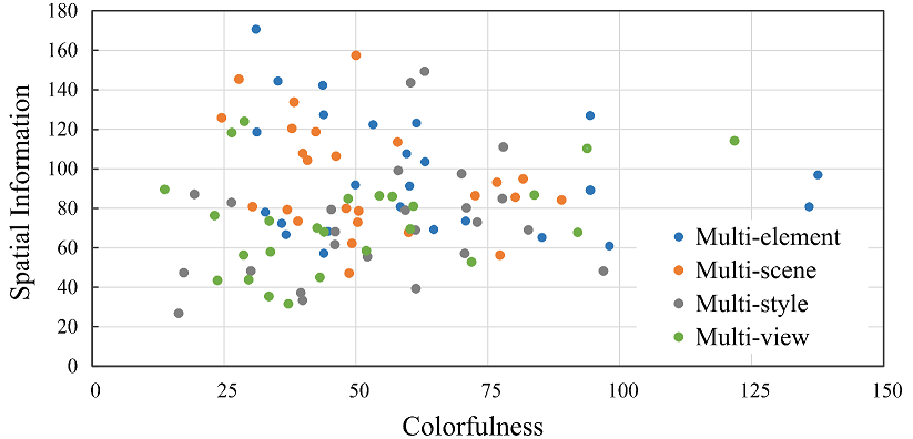
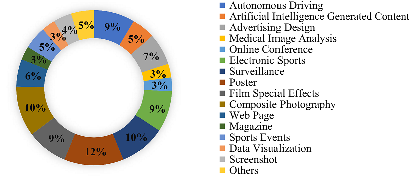
We provide some statistical data on our ciCIQA database, as shown in Fig.3. The diversity of images is measured in terms of spatial information and colorfulness. The top provides the scatter plot of the spatial information and colorfulness of ciCIQA. As seen, the scatter is distributed across the entire range, which indicates the composition of our database samples is reasonable. The bottom presents the statistical proportion of different applications. As seen, the raw data of ciCIQA comes from more than 15 application scenarios. Therefore, we believe that the collected images can well represent the overall space of CIs.

(a) The scatter plot of spatial information (or content diversity) and colorfulness

(b) The statistical proportion of images that comes from each application scenario in a sunburst chart
Fig.3: Statistical properties of the proposed ciCIQA database.

(1.2) Generation of Compressed CI Samples. To generate compressed CI samples with various encoders, we employ four video compression standards (e.g., A V1, H.264/A VC, H.265/HEVC, and H.266/VVC) and two widely-used image compression standards (e.g., JPEG and WebP). Among them, H.266/VVC is the latest video coding standard. The detailed compression settings are summarized as follows:

a) AV1. We utilize the libaom-av1 encoder in FFmpeg 4.2.4 for A V1 encoding. The encoding command is set as: "ffmpeg -s 1920x1080 -pix fmt yuv420p -i input file c:v libaom-av1 -crf xx -b:v 0 output file", where -s refers to the resolution of the output file, -c:v specifies the video encoding library is libaom-av1, and -crf refers to the constant rate factor (CRF), which is the quality control parameter. The CRF value (i.e., denoted by "xx") is adjustable within the range of 0 to 63, where selecting lower values leads to enhanced video quality but larger file sizes.

b) H.264/AVC. Similar to AV1, we use libx264 in FFmpeg 4.2.4 for H.264 encoding. The encoding command is set as: "ffmpeg -s 1920x1080 -pix fmt yuv420p -i input file c:v libx264 -qp xx output file", where -qp represents the quantization parameter (QP). QP serves as the quality control factor, and it accepts a value ranging from 0 to 51 in the experiments.

c) H.265/HEVC. We employ the libx265 in FFmpeg 4.2.4 for H.265 encoding. Similar to H.264, the encoding command is set as: "ffmpeg -s 1920x1080 -pix fmt yuv420p -i input file -c:v libx265 -qp xx output file".

d) H.266/VVC. We use VTM 14.2 and the main profile for H.266 encoding with the same quality control parameters as H.264. The related encoding command is set as: "EncoderApp.exe -c encoder intra vtm.cfg -i input file -q xx -o output file -b bin file", where -c specifies the configuration file as encoder intra vtm.cfg.

e) JPEG. The MATLAB function "imwrite" implements the JPEG compression. The compressed images at different quality levels are controlled by quality factor (QF), which can be adjusted within the range of 0 to 100. A larger QF value means a better quality, and vice versa.

f) WebP. We employ the libwebp in FFmpeg 4.2.4 for WebP encoding. The encoding command is set as: "ffmpeg -s 1920x1080 -pix fmt yuv420p -i input file -c:v libwebp -quality output file", where -quality denotes a QF parameter used to control the compression quality, with values ranging from 0 to 100.

As is well known, when QP or CRF is too small (i.e., QF is too large), the quality difference between the compressed and original images is almost indistinguishable. In contrast, when QP or CRF is too large (QF is too small), the visual quality of a compressed image can be very annoying. Based on the prior experience, we set the QP and CR values range between 23 and 47, and the QF value ranges between 5 and 70 to save labor costs, respectively. Consequently, a total of 23200 compressed images are generated for subjective experiments.

(2) Annotation of Compressed CI Samples.

Existing studies have shown that human perceptual quality can be represented as a step function of QPs, where perceived quality remains constant between two adjacent perceptual quality jump points (i.e., JND points). In other words, they can be used to guide an encoder to select the maximum QP that ensures the compressed image belongs to the same visual quality level. Therefore, when manually annotating the compressed CI samples, it is of great significance to determine the best jump point that human eyes can not distinguish the difference between two QPs with the largest gap.

(2.1) Annotating Just Noticeable Difference (JND). To annotate consecutive visual quality, we have conducted subjective experiments to annotate the first five JND points for each CI sample, and the overall settings are similar to [Wang2016JVCIR]. Specifically, we have employed a double stimulus and designed a graphical user interface for the JND subjective experiments. We have invited 20 participants (9 females and 11 males with no background in image processing) to compare two images displayed side by side. Participants are asked to select "Yes" or "No" to indicate whether there is a quality difference between two juxtaposed images. Considering the limited number of testing images and time constraints, we employed a binary search method to expedite the search for the jump points. Table II summarizes the main information about the experimental conditions and parameter configurations.

Fig.4: Illustration of consecutive quality levels and the first five perceptual jump points of JPEG and H.266/VVC. The blue dot line represents the quality curve, and the orange solid line represents a step function of the related jump points on our ciCIQA.

Fig.5: Distribution of different visual quality levels. The average quantization value is calculated for each compression standard. To ensure the consistency of illustrations, we subtract the relevant quantization value (i.e., QF) from 100 in JPEG and AV1.

(2.2) Annotating Visual Quality Score (VQS): To annotate the visual quality scores (VQSs) for each CI sample at five jump points, we further employ a single stimulus and design a graphical user interface to carry out the subjective experiments. Specifically, we have invited 21 participants including 12 females and 9 males. Each subject is asked to score the image quality based on 11 discrete quality scores ranging from 0 to 1 with a step length of 0.1, which corresponds to five quality levels (i.e., [0,0.1] for bad, [0.2,0.3] for poor, [0.4,0.5] for fair, [0.6,0.7] for good, and [0.8,1.0] for excellent, as suggested in [ITU2020]). Other details are provided in Table II.

Fig.6: Histogram of the MOS values on our ciCIQA database.

Fig.7: Histogram of the confidence interval for subjective ratings on our ciCIQA database.

(3) Processing of Subjective Experimental Results.

To ensure the validity of the subjective experimental data, we have performed the outlier detection and the observer rejection before using the annotated samples obtained from two subjective experiments. For the JND subjective experiments, we use the same outlier detection method as suggested in [Shen2021TIP].

For the VQS subjective experiments, we calculate the confidence interval of the VQS results at the confidence level of 95% [46]. In particular, we obtain the mean µ and the standard deviation δ of all subjective results. For example, the confidence interval of the i-th CI sample is defined as , where Nob denotes denotes the total number of observers. If the subjective label exceeds the corresponding confidence interval, the related annotation is considered as an outlier. When the number of outliers for a subject exceeds a certain threshold (i.e., 18 in our experiments), all the annotations from that subject are discarded as suggested in [Xiang2020TMM]. Based on the above outlier processing, two subjects were rejected in our experiments.

(4) Statistical Analysis of ciCIQA.

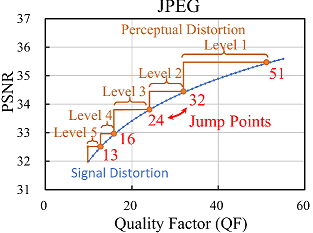
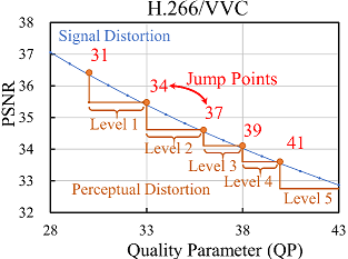
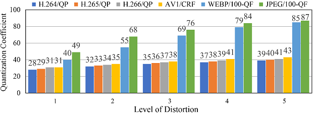
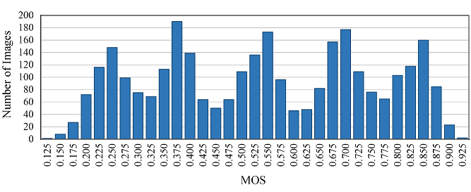
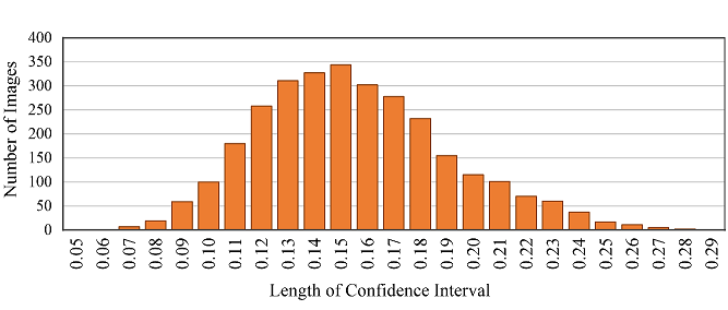
The HVS prior knowledge tells us that human eyes barely discern subtle compression distortion differences. To improve the compression efficiency, we can encode a CI sample with the maximum QP between two adjacent jump points. We calculate the average results of the first five jump points on our ciCIQA database, and show the statistical results of JPEG and H.266/VVC in Fig.4. The blue dotted line represents the compression distortion in terms of signal distortion, while the red solid line represents the compression distortion in terms of perceptual distortion. As seen, HVS can perceive the consecutive quality level over discrete QPs from lossless to severe signal distortion. It also reveals that we can choose more suitable encoding parameters (i.e., QP) under the same perceptual quality to reduce storage and bandwidth requirements. Fig.5 provides the distribution of visual quality levels for six different encoders. Based on this statistical distribution, we have observed an interesting consistent trend: as the perceptual quality level gradually decreases (i.e., higher visual quality), the change rate of quantization value progressively increases. In other words, when the image quality increases to a certain level, it is difficult for human eyes to detect changes in finer details. The fundamental reason behind this trend is that HVS has limited resolutions, because it can be affected by physiological structure (e.g., retina cell types and quantity) and cognitive process (e.g., knowledge and experience). These statistics provide valuable insights that help us better understand and achieve a balance between image quality and compression ratio, showing useful guidance for the development of composite image compression. Fig. 6 provides the distribution of MOSs, covering the entire range of visual quality. It demonstrates that ciCIQA includes a diverse set of compression distortion samples across various quality levels, and the boundaries between different quality levels are also easily discernible. Furthermore, upon closer inspection, the histogram of the MOS values shows five distinct peaks, which is consistent with the construction strategy in our database, where the distortion level is determined by the first five JND points. Furthermore, we have validated the consistency among all subjects by calculating their mean and standard deviation of the rating scores and maintaining a confidence level of 95% [ITU2020]. As illustrated in Fig. 7, we report the lengths of the confidence interval for subjective ratings of all images. As seen, these confidence interval lengths are primarily distributed between 0.10 and 0.21. This suggests that there is a high level of consistency among the subjective ratings in our ciCIQA. As a result, the MOS results obtained from the subjective experiments are reliable for the CIQA task

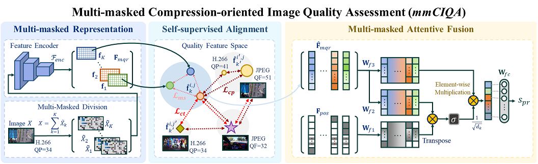
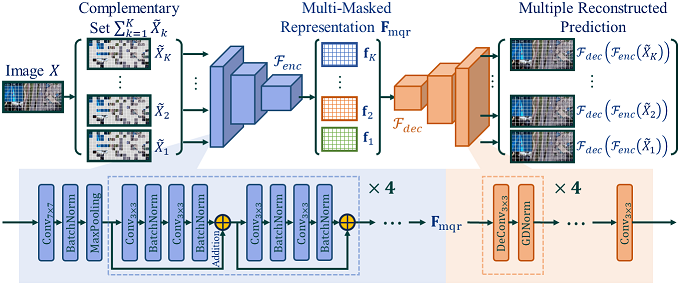
Existing compression standards typically adopt a block-level coding paradigm, dividing the input image into no-overlapping blocks and encoding them separately. The compression process for each block is similar, and all decoded blocks contribute to the image-level quality experience. As a result, we believe that the characteristics of compression distortion can be effectively captured at the block level. Inspired by this, we propose a new multi-masked no-reference CIQA metric, where we focus on extracting quality relationship features between different blocks through randomly masking and learning the encoding distortion features at the block level. mmCIQA mainly consists of three modules, including 1) multi-masked quality representation, 2) self-supervised quality alignment, and 3) multi-masked attentive fusion as shown in Fig. 8.

Fig.8: Pipeline of the proposed multi-masked CIQA model (i.e., mmCIQA).

(1) Multi-masked Quality Representation.

Multi-masked quality representation aims to learn CI features to describe their perceived compression quality. In general, the content variations of each image block and different encoders result in different perceptual visual quality. It indicates that compression distortions appeared in each block tend to be relatively independent. On the other hand, the compression quality of each block jointly affects the visual quality of an entire image. To better represent the compression quality features, we design a task to learn from randomly masked CI images. Through this task, we aim to guide a trained model to learn the characteristics of the compression distortion within a block and the quality relationship between different blocks, as illustrated in Fig. 9.

Fig.9: Illustration of multi-masked quality representation.

(2) Self-supervised Quality Alignment.

Compression distortions demonstrate subtle differences, posing a challenge for the aforementioned reconstruction task to learn the quality representation of CIs. In order to better represent the quality differences on different encoders (e.g., JPEG, A V1, and H.266/VVC) and different compression settings (e.g., QPs), we design a self-supervised quality alignment method as follows.

Specifically, we adopt a self-supervised triplet feature metric to measure the feature difference, including compression-based hard contrast, content-based hard contrast, and block region-based soft contrast. Given $X^{i,j}$ from the i-th compression operation (e.g., parameter settings and encoder types) and the j-th original CI sample, the corresponding k-th feature is ${\mathbf{f}}_k={\mathcal{F}}_{Enc}({\tilde{X}}_k^{i,j};{\theta }_{Enc})$. Furthermore, we employ a spatial average pooling AvgPool2D followed with one 1x1 convolution Conv to obtain 128-dimensional aligned features ${\hat{f}}_k^{i,j}$.

(3) Multi-masked Attentive Fusion.

Considering that the block location also affects visual perception, we need to preserve the latent spatial location of feature elements when integrating multi-masked features. Therefore, we propose a multi-masked attentive fusion method, which integrates all features by a masking-based spatial position embedding and a cross-attentive fusion.

Table.2: Performance comparison of some representative QA methods.

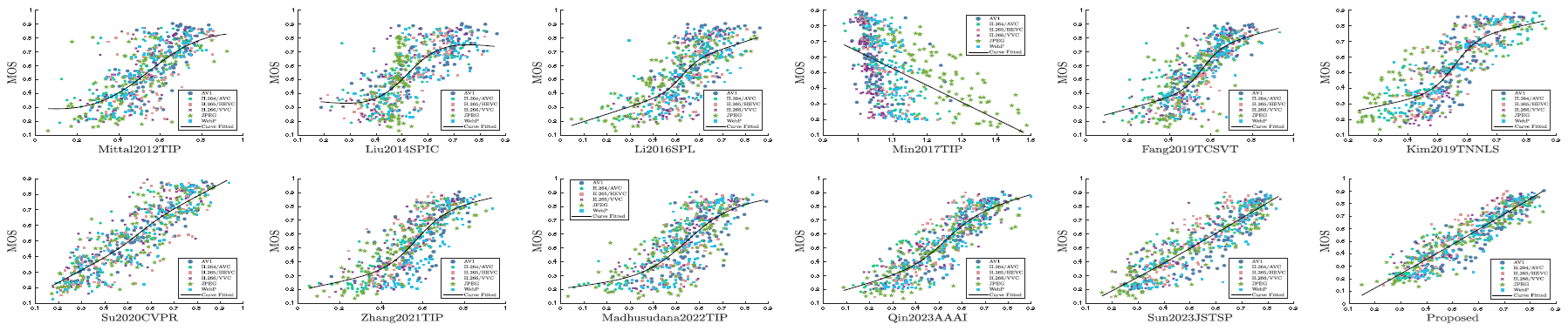
Visual Comparison via Scatter Plots. To better visualize and compare the overall prediction distributions, we use scatter plots and fitting curves predicted by different IQAs, as shown in Fig. 10. The scatter plots in each figure are represented by six different shapes, representing the predicted results with different compression standards, while the solid fitted curve represents the average trend of the predicted results. For nonlinear fitting, the closer the scatter points are to the fitting curve, the better the prediction performance. As seen, the scatter points of our mmCIQA are more concentrated around the fitting curve, indicating that it has more consistent predicted scores with visual quality.

Fig.10: Scatter plots of 12 NR methods on the proposed ciCIQA database. Six different colors are used to distinguish six different compression standards. The black solid line curve is a non-linear fitting of the quality scores predicted by each method.